Biplot of a spatial PCA

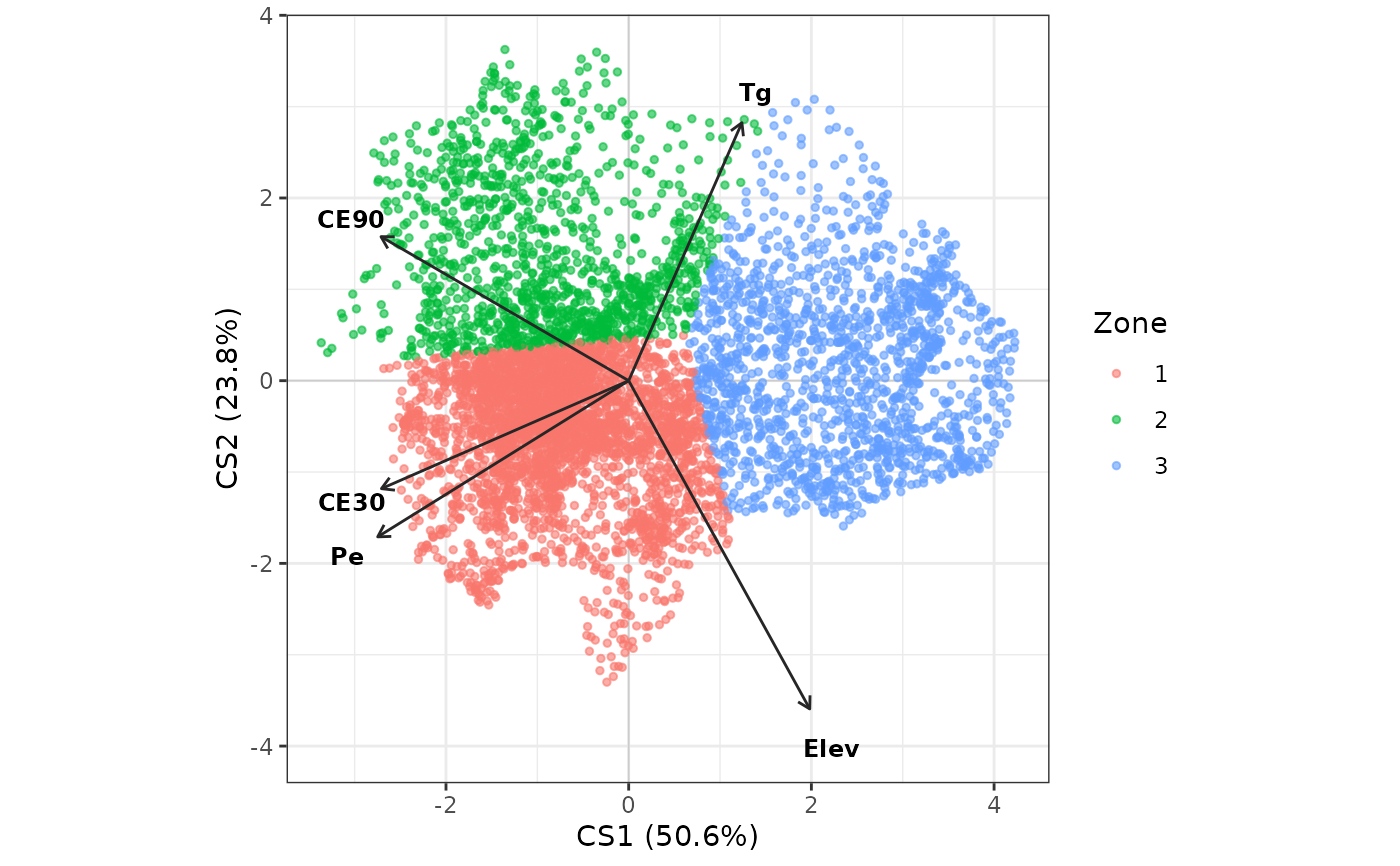
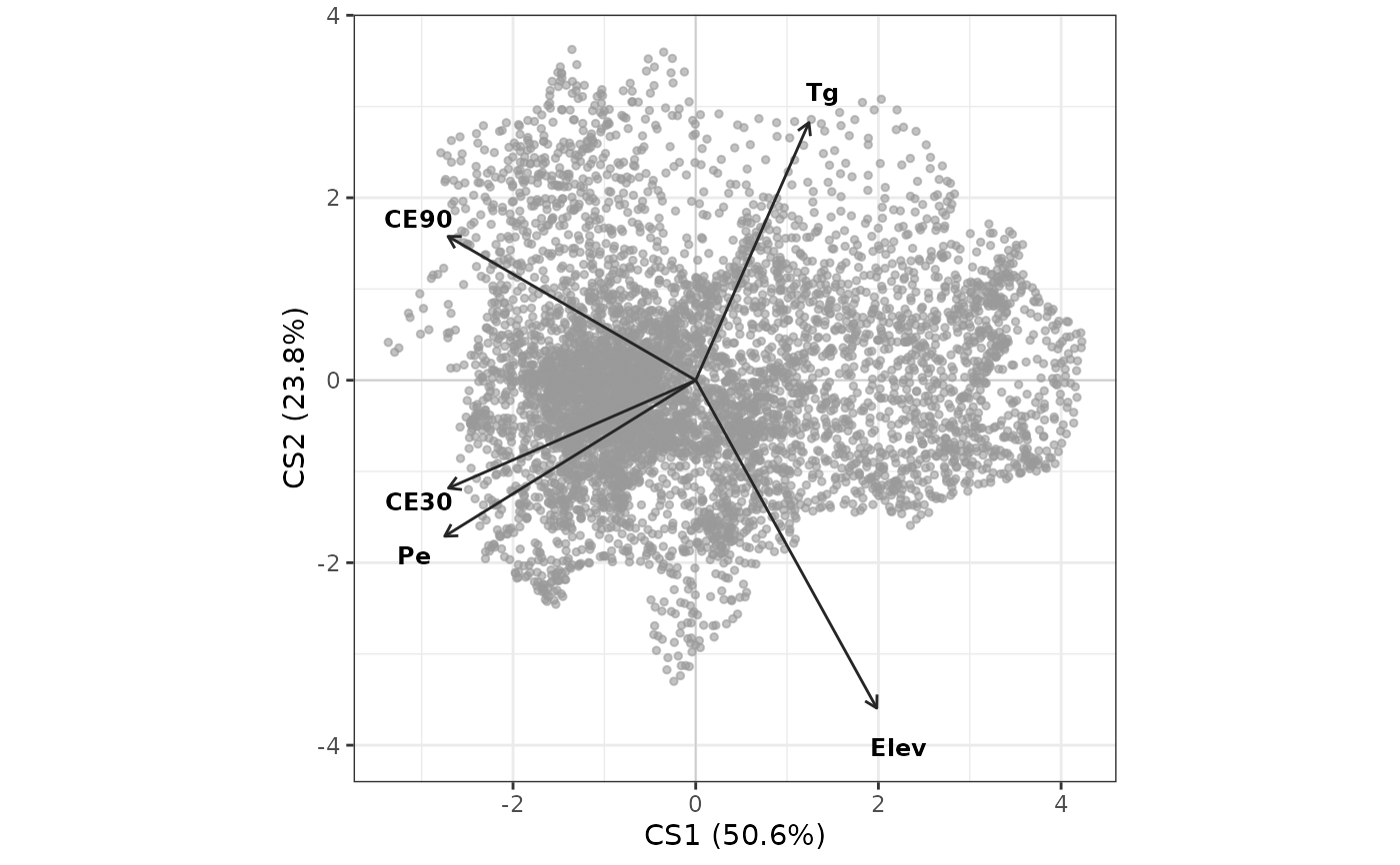
Builds a biplot from the spatial principal component analysis computed by [kmspc()]. Sites are drawn as points using their coordinates on the retained spatial components, and variables as arrows from the origin using their loadings.

The biplot complements the clustering output: the angles between arrows approximate the correlations among the original variables, the length of an arrow indicates how well the plotted plane represents that variable, and the position of a site relative to an arrow indicates its relative value for that variable. When management zones are mapped onto the points, it also shows which variables drive the separation between zones.

Usage

spca_biplot(
  x,
  axes = c(1, 2),
  cluster = NULL,
  arrow_scale = NULL,
  point_size = 1,
  point_alpha = 0.6,
  label_size = 3.2
)

Arguments

x

a list returned by [kmspc()].

axes

numeric vector of length two with the spatial components to be plotted.

cluster

optional. Either a character with the name of one of the columns of x$cluster (for example "Cluster_3"), or a vector with one value per site. Points are coloured according to it.

arrow_scale

numeric. Factor applied to the loadings so that the arrows are legible next to the cloud of sites. If NULL (default) it is computed so that the longest arrow spans about 85% of the point cloud. Because the same factor is applied to every arrow, it does not alter their interpretation.

point_size, point_alpha

numeric. Size and opacity of the points.

label_size

numeric. Size of the variable labels.

Value

A ggplot object, which can be further modified with the usual ggplot2 functions.

Details

Note that the sign of a component is arbitrary: the eigendecomposition fixes the direction of each axis but not its orientation, so two runs may produce mirrored biplots without any change in the conclusions. Interpretations should therefore be phrased in terms of relative positions, that is, which variables oppose each other and which go together, rather than in terms of absolute signs.

The correlations suggested by the angles between arrows are computed treating the sites as independent observations. With spatially autocorrelated layers that assumption does not hold, so the magnitudes remain a valid description of the observed association but their statistical significance is misleading. See [spatial_t_test()] for a test that corrects the degrees of freedom by the effective sample size.

See also

[kmspc()], [spatial_t_test()]

Examples

library(sf)
data(wheat, package = 'paar')

# Transform the data.frame into a sf object
wheat_sf <- st_as_sf(wheat, coords = c('x', 'y'), crs = 32720)

# Run the kmspc function
kmspc_results <- kmspc(wheat_sf, number_cluster = 2:4)
#> Warning: All numeric Variables will be used to make clusters

# Biplot of the first two spatial components
spca_biplot(kmspc_results)


# Colouring the sites by the three-zone classification shows which variables
# drive the separation between management zones
spca_biplot(kmspc_results, cluster = "Cluster_3")