Getting started with ofemeantest • ofemeantest

ofemeantest implements a cell-based, permutation-based protocol to compare treatments in unreplicated on-farm experiments (OFE) where strips of management are laid out side-by-side over a field and yield is recorded densely (e.g., from a yield monitor).

The package handles three things:

Build a regular grid over the trial and aggregate the dense point data into cell-level medians, keeping only cells that fall inside a single treatment strip and contain enough observations.
Estimate the effective sample size (ESS) from the spatial autocorrelation of the residuals of a one-way ANOVA on cell medians, to avoid pseudo-replication from spatially correlated data.
Test treatment differences with a permutational ANOVA, repeated over many random subsamples of size ESS, and report the median p-value as the field-specific test result.

Installation

# install.packages("pak")
pak::pkg_install("PPaccioretti/ofemeantest")

A worked example

The bundled ofe_f2 dataset comes from a corn (Zea mays L.) trial where a single fertilized strip (~2.2 ha) was compared against an adjacent control strip on the same field. Raw yield-monitor data were cleaned following Vega et al. (2019).

library(ofemeantest)
data("ofe_f2")

head(ofe_f2)
#>    Treatment Yield_tn                geom
#> 1 Fertilized 7.915459 388594.8, 6370076.9
#> 2 Fertilized 7.984485 388595.5, 6370078.5
#> 3 Fertilized 6.685809 388596.3, 6370080.2
#> 4 Fertilized 6.265568 388597.2, 6370081.8
#> 5 Fertilized 5.508421     388598, 6370083
#> 6 Fertilized 4.486158 388598.8, 6370085.0

Quick run

Call ofemt() and let it build the grid internally:

res <- ofemt(
  data = ofe_f2,
  y = "Yield_tn",
  x = "Treatment",
  cellsize = 9,
  min_per_cell = 4,
  n_p = 2000,
  n_s = 200,
  alpha = 0.05
)
res
#> 
#> === OFE permutation analysis ===
#> Cellsize: 9 x 9 | Total cells: 1840 | Selected cells: 554
#> Obs/cell (min/median/max): 4 / 5 / 7
#> n: 554 | ESS: 97 | Rho: 0.652 | Moran's I: 0.548
#> 
#> --- Means comparison (sorted by decreasing mean) ---
#>   Treatment Yield_tn_mean letters
#>  Fertilized      5.280402      a 
#>     Control      4.760095       b
#> 
#> --- Pairwise tests (median p across runs) ---
#>              Comparison p_value  p_adj
#>  Fertilized vs. Control  0.0055 0.0055

Key fields in the printed result:

Selected cells: cells retained after filtering by single treatment and min_per_cell.
n / ESS: nominal sample size and effective sample size given the spatial autocorrelation of the residuals.
Rho / Moran’s I: spatial autocorrelation indicators.
Means comparison: per-treatment median yield (in cells) and compact letter display from the multiple-comparison procedure.
ANOVA permutation test: median p-value per pairwise comparison.

Step-by-step

For finer control — inspecting the grid, tweaking the cell size, or reusing the same selection in several downstream analyses — build the grid explicitly with make_ofe_grid() and pass it to ofemt().

g <- make_ofe_grid(
  data = ofe_f2,
  x = "Treatment",
  cellsize = 9,
  min_per_cell = 4
)
names(g)
#> [1] "grid_all"   "grid_sel"   "params"     "cell_stats"


plot_grid_selection(g, data = ofe_f2)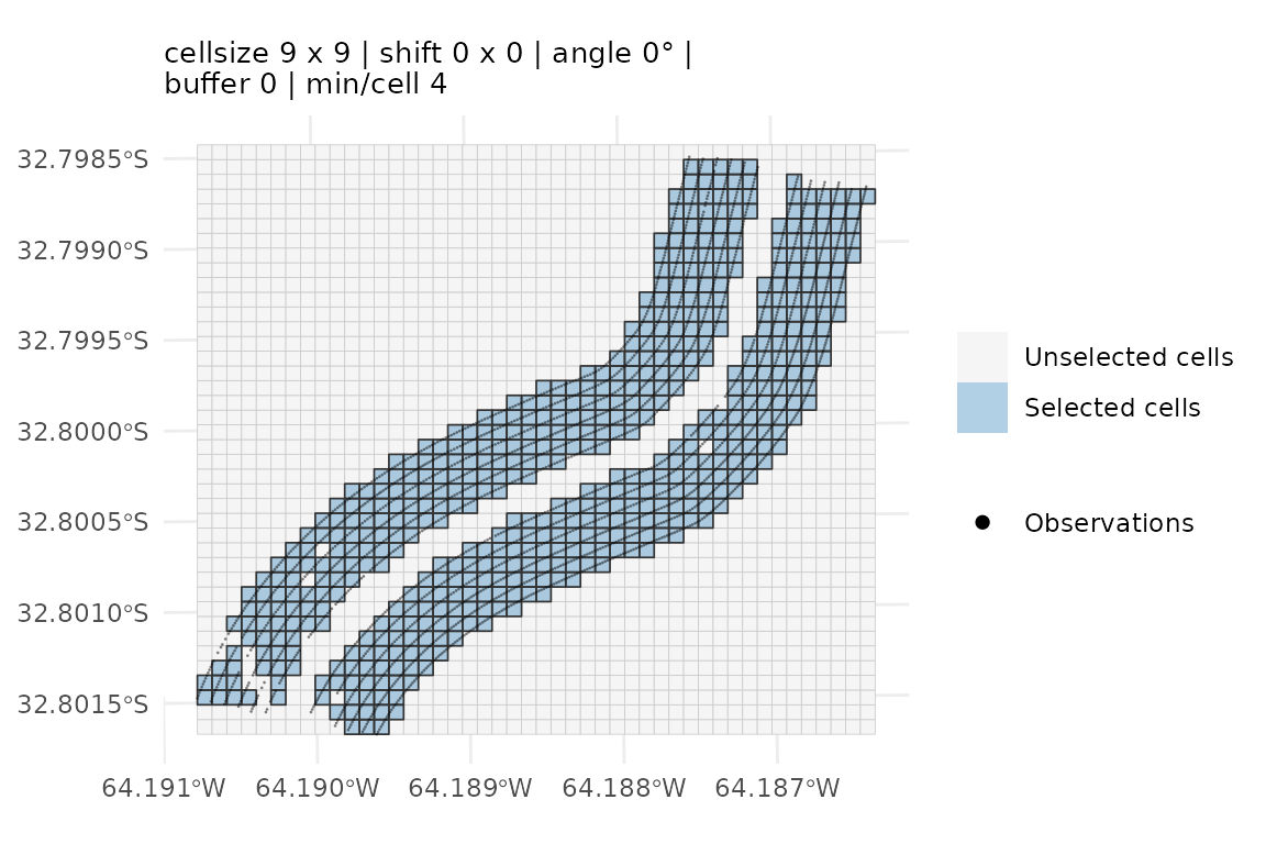


res2 <- ofemt(
  data = ofe_f2,
  y = "Yield_tn",
  x = "Treatment",
  grid = g,
  n_p = 2000,
  n_s = 200
)

Both calls produce the same numeric output when the grid is built with matching arguments — ofemt(grid = NULL, ...) is equivalent to ofemt(grid = make_ofe_grid(...)) under the hood.

Tuning the grid

plot_grid_selection() draws the three layers on one set of axes: the full grid in grey, the cells that survived the filters shaded in blue, and the observations as points. Overlaying the points on the cell boundaries is what makes the geometric arguments legible — a cell is dropped either because it straddles two treatments or because too few points landed inside it, and both are visible at a glance.

By default the plot is built with ggplot2, which keeps the legend outside the panel — it can never land on top of the data, and the result does not change with the size of the graphics device. Pass engine = "base" for base graphics instead; if ggplot2 is not installed, that is what you get anyway, with a message. Because the ggplot2 engine returns a ggplot object, you can keep customising it:

plot_grid_selection(g, data = ofe_f2) +
  ggplot2::labs(subtitle = "Lote 2, campaña 21/22")

plot_grid_selection(g, data = ofe_f2, engine = "base")

With dense yield-monitor data the observations can swamp the cell boundaries; lower point_size until the grid shows through.

The title of each plot repeats the parameters used, so successive calls can be compared directly:

op <- par(mfrow = c(1, 2))
plot_grid_selection(
  make_ofe_grid(ofe_f2, x = "Treatment", cellsize = 9, min_per_cell = 4),
  data = ofe_f2
)
# Shift the origin by half a cell and rotate to follow the strips
plot_grid_selection(
  make_ofe_grid(
    ofe_f2,
    x = "Treatment",
    cellsize = 9,
    min_per_cell = 4,
    shift = c(4.5, 4.5),
    angle_deg = 10,
    buffer = 5
  ),
  data = ofe_f2
)
par(op)

Keeping the geometries in the result

By default ofemt() returns tables only. Set keep_components to embed the spatial objects in the result, which lets you plot the analysis that actually ran rather than rebuilding the grid by hand:

`keep_components`	Adds to the result	`plot()` shows
`"none"` (default)	nothing	(errors — no geometries)
`"light"`	`grid`, the full `ofe_grid` (`grid_all`, `grid_sel`, `cell_stats`, `params`)	grid + selected cells
`"full"`	`"light"` plus `cell_medians` (one point per selected cell, with its median response and ANOVA residual) and `points_joined` (every observation with its `CellID`)	grid + selected cells + points

Cost scales accordingly: "light" stores one polygon per grid cell, "full" adds one row per observation.

res_full <- ofemt(
  ofe_f2,
  y = "Yield_tn",
  x = "Treatment",
  cellsize = 9,
  min_per_cell = 4,
  keep_components = "full"
)

# No further arguments needed — every layer comes from the object itself
plot(res_full)

# The per-cell medians and residuals that fed the spatial diagnostics
head(res_full$cell_medians)

Reproducibility

ofemt() exposes a seed argument that controls the random subsampling inside the permutation runs. The default is seed = 7L, so two calls with the same inputs return identical p-values:

identical(
  ofemt(
    ofe_f2,
    y = "Yield_tn",
    x = "Treatment",
    cellsize = 9,
    min_per_cell = 4,
    seed = 7L
  ),
  ofemt(
    ofe_f2,
    y = "Yield_tn",
    x = "Treatment",
    cellsize = 9,
    min_per_cell = 4,
    seed = 7L
  )
)
#> TRUE

Pass seed = NULL to let results vary across runs (e.g., when exploring sensitivity to the random draws).

Inspecting the permutation distribution

Each call retains the per-run p-values in res$perm_runs so you can sanity-check that the median p-value is not an artefact of a long tail. perm_runs has one row per comparison per sampling run, with columns Comparison, p_value (that run’s permutation p-value), p_adj (the same value after adjusting for multiplicity within the run) and run.

plot_pvalue_hist() draws that distribution with two reference lines per panel: a solid line at the median — the value reported in the ANOVA permutation test table — and a dashed line at alpha.

# Requires the optional 'ggplot2' package.
plot_pvalue_hist(res)

When the analysis was run with a multiplicity adjustment, the histogram shows the adjusted values by default, so the median line and the reported p_adj always refer to the same quantity. Use which = "raw" to see the unadjusted distribution instead:

res_bonf <- ofemt(
  ofe_f2,
  y = "Yield_tn",
  x = "Treatment",
  cellsize = 9,
  min_per_cell = 4,
  p_adjust_method = "bonferroni"
)

plot_pvalue_hist(res_bonf) # adjusted
plot_pvalue_hist(res_bonf, which = "raw") # unadjusted

Where to go next

vignette("methodology") — technical description of the protocol (effective sample size, permutational ANOVA, multiplicity adjustment).
?ofemt — full argument reference for the main function.
?make_ofe_grid — details on grid construction and selection.

References

Córdoba, M., Paccioretti, P., & Balzarini, M. (2025). A new method to compare treatments in unreplicated on-farm experimentation. Precision Agriculture, 26(1), 4. https://doi.org/10.1007/s11119-024-10206-0
Griffith, D.A. (2005). Effective geographic sample size in the presence of spatial autocorrelation. Annals of the Association of American Geographers 95(4): 740–760.
Vega A., Córdoba M., Balzarini M. (2019). Protocol for automating error removal from yield maps. Precision Agriculture 20: 1030–1044. https://doi.org/10.1007/s11119-018-09632-8